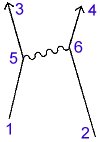
This diagram shows three basic actions. The first, a photon goes from place to place, is illustrated by the line from 5 to 6. The second, an electron goes from point A to point B in space-time, is illustrated by the lines from 1 to 5, 5 to 3, 2 to 6, and 6 to 4. The third, an electron emits or absorbs a photon, is illustrated by the junctions at points 5 and 6.
So in simple terms, what does this diagram depict? It shows an electron, which starts out at 1 and moves through time-space to point 5, where it emits a photon, altering its path and moving along to point 3 where it goes off of the graph. Another electron starts out at point 2 where it travels through space-time to point 6 and absorbs the photon emitted by the first electron. Its path changes and it travels to point 4 where it leaves the graph.
And for those who want a bit more detail…
Illustrated above is an animated Feynman Diagram depicting the three basic actions which can occur. Along the y-axis (up and down) is the time scale. Since we will be dealing with photons and electrons, which move very rapidly, a 45 degree angle represents something going the speed of light (the squiggly line). The x-axis (left and right) represents space. All of the particles (both the electrons (![]() ) and the photon (
) and the photon (![]() )) represented in the diagram move through time and space.
)) represented in the diagram move through time and space.
Now, let’s look at the first basic action in detail – a photon goes from place to place. (This is illustrated above a wiggly line for no good reason – it is just an arbitrary depiction.) More accurately, it should be said that a photon is known to be at a given place at a given time and has a certain amplitude to get to another place at another time. There is a formula for the size of this line. It is one of the great laws of Nature, and it’s very simple. It depends on the difference in distance and the difference in time between the beginning and ending points of the line. These differences can be expressed mathematically as (X2 – X1) and (T2 – T1). (You may recognize this as part of the Pythagorean Theorem – which in this case would actually involve three terms representing the x, y, and z-axis.)
The major contribution to the size of the arrow (which we call P(A to B)) occurs at the conventional speed of light – when (X2 – X1) is equal to (T2 – T1) – where one would expect it all to occur, but there is also an amplitude for light to go faster (or slower) than the conventional speed of light. Light doesn’t go only in straight lines nor does it always go only at the speed of light!
It may surprise you that there is an amplitude for a photon to go at speeds faster or slower than the conventional speed, which is called c. The amplitudes for these possibilities are very small compared to the contribution from speed c; in fact, they cancel out when light travels over long distances. However, when the distances are short these other possibilities become vitally important and must be considered.
The second action fundamental to quantum electrodynamics is: an electron goes from point A to point B in space-time. (For the moment we will imagine this electron as a simplified, fake electron, with no polarization – what the physicists call a “spin-zero” electron. In reality, electrons have a type of polarization, which doesn’t add anything to the main ideas; it only complicates the formulas a little bit.) The formula for the amplitude for this action, which we will call E(A to B) also depends on (X2 – X1) and (T2 – T1) as well as on a number we will call n, a number that, once determined, enables all our calculations to agree with experiment. It is a rather complicated formula, and the really isn’t a way to explain it in simple terms. However, you might be interested to know that the formula for P(A to B) – a photon going from place to place in space-time – is the same as that for E(A to B) – an electron going from place to place – if n is set to zero.
The third basic action is: an electron emits or absorbs a photon – it doesn’t make any difference which. We will call this action a “junction” or “coupling.” (This is the point where the squiggly and straight lines meet in the diagram above.) To distinguish electrons from photons in the diagrams, electrons will be depicted going through space-time as a straight line. Every coupling, therefore, is a junction between two straight lines and a squiggly line. There is no complicated formula for the amplitude of an electron to emit or absorb a photon; it doesn’t depend on anything – it’s just a number!
Adapted from QED – The Strange Theory of Light and Matter by Richard P. Feynman (Princeton University Press, 1985)
These diagrams are roadmaps for calculating how things happen in nature – and they don’t happen in just one way: for example, two electrons going from one place to another in spacetime can happen in several different ways:
1. Just two straight lines, no photons emitted or absorbed. This accounts for something like a 99% agreement between the calculated probabilities and the actual probabilities as observed in experiment. But Feynman could calculate better than that.
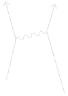
2. The diagram as shown above. Note: the photon (a “virtual photon”) is not actually detected going from one electron to the other – indeed, it could be imagined as a positron going backwards in time, and it wouldn’t make any difference in the numbers. By taking into account this additional possibility, the calculated probability better matches the observed probability in experiment.
3. The diagram as shown, but with the (virtual) photon disintegrating into a positron-electron pair, annihilating into a new photon, and getting absorbed into the other electron. Again, none of the supposed activity in the middle of the diagram is observed, but by calculating these additional possibilities, the theoretical numbers match even MORE closely the probabilities observed in experiment.
4. You could also have a diagram with two photons being emitted and absorbed, or a diagram in which one photon goes out and back into the electron on the left, and the other photon goes out from the left electron and across to the photon on the right. There are many, many different ways this can happen, and the diagrams are a shorthand for showing categories of possibilities.
Feynman often wondered aloud something along these lines: how do the electrons and photons KNOW how to calculate all these possibilities, which we and our big supercomputers can only barely begin to calculate?